Gnome: A Gauss–Newton optimizer for sciml.
Empirical Fisher based optimizers, like adam and SOAP, struggle with MSE. Gnome is a targeted fix.
Code, experiments, and everything needed to reproduce this post: github.com/tmayer868/gnome-optimizer.
AdamW, the default optimizer in deep learning, can’t fit a linear regression. Run it at a fixed learning rate and it never reaches the minimum — it gets within a ball of radius \(\sim\eta\) of the solution and rattles around in there forever. SOAP, which has shown SOTA performance in PINNs, inherits the same failure. The standard fix — decay the learning rate to zero on a schedule — doesn’t repair anything; it forces the steps to zero on a clock and hopes you guessed the horizon right.
My thesis is that if you can’t trust an optimizer with linear regression, you can’t trust it with any regression. OLS is the friendliest optimization problem there is — convex, smooth, closed-form answer — and the rare case where you can measure exactly how wrong the final parameters are instead of squinting at a loss curve. An optimizer that needs a babysitter here needs one everywhere; it’s just harder to catch.
This post shows the failure and traces it to two defects of the Adam/empirical-Fisher family, each one equation long:
- Step size. \(\mathbb E[\hat g^2] = \mathbb E[g]^2 + \tfrac{1}{B}\operatorname{Var}[g]\) — neither term is curvature: the first cancels against the numerator (sign-steps), the second is a noise floor set by the batch size \(B\). With or without the square root, whether the step anneals is an accident of local signal-to-noise, never a measurement of arrival.
- Basis. \(\sum_k g_k g_k^\top = 4\sum_k r_k^2\, J_k^\top J_k\) — the empirical Fisher is the Gauss–Newton matrix with every sample reweighted by its squared residual, so outliers vote quadratically and the eigenbasis tracks your worst errors, not the curvature.
Gnome (Gauss-Newton optimizer via matrix eigendecomposition) modifies SOAP with one fix per defect: it replaces SOAP’s empirical-Fisher curvature approximation with an unbiased estimate of the generalized Gauss–Newton matrix (the basis), and it takes a clipped Newton step in the rotated basis instead of an Adam step (the step size). The result is a step size that goes to zero because the residual does, not because a schedule said so.
Here’s the headline before the argument — physics-informed neural network (PINN) benchmarks, final error against a reference solution, Gnome at a fixed learning rate versus baselines given warmup plus a tuned cosine decay to zero:
| benchmark | metric | Gnome (fixed LR) | SOAP (cosine → 0) | AdamW (cosine → 0) | best baseline ÷ Gnome |
|---|---|---|---|---|---|
| Poisson | rel. \(L_2\) | 2.3e-5 | 2.7e-4 | 8.4e-4 | 12× |
| val. loss | 2.1e-9 | 3.6e-7 | 4.6e-6 | 175× | |
| Burgers | rel. \(L_2\) | 2.7e-5 | 1.0e-4 | 4.8e-4 | 3.8× |
| val. loss | 7.2e-8 | 6.3e-7 | 4.6e-6 | 8.7× | |
| Kuramoto–Sivashinsky | rel. \(L_2\) | 7.0e-2 | 4.7e-1 | 4.8e-1 | 6.7× |
| val. loss | 1.2e-6 | 6.2e-4 | 6.7e-4 | 502× |
None of these runs use the PINN bag of tricks: no causal weighting, no NTK- or gradient-norm-based loss balancing, no Fourier features, no adaptive collocation resampling (RAR), no hard boundary-condition enforcement, no curriculum training, no modified-MLP architectures. Every run is a plain MLP with fixed loss weights. The only variable is the optimizer.
The rest of this post is the explanation of that table, built up from the smallest problem that shows the mechanism.
1. A test every optimizer should pass: ordinary least squares
Fit a linear model \(\hat y = X\beta\) under squared error, \(\mathcal L(\beta) = \tfrac1N\lVert X\beta - y\rVert^2\). This is the friendliest optimization problem there is: it is convex, smooth, and has a unique closed-form minimizer,
\[ \beta^\star \;=\; (X^\top X)^{-1} X^\top y . \]
There is a single right answer, and we can compute it directly. So we can ask an optimizer the most exacting question there is: after training, how far is your \(\beta\) from \(\beta^\star\)? Not “how low is the loss” — how close is the actual solution.
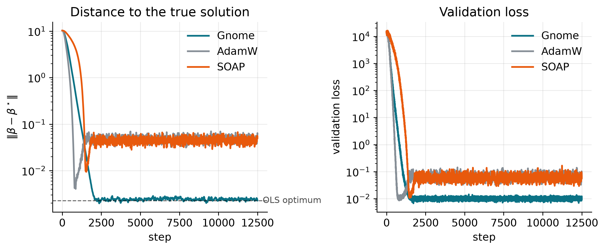
Here are Gnome, AdamW, and SOAP on a 64-feature least-squares problem (condition number \(10^3\)), each run at a fixed learning rate. The left panel is the distance to the true solution \(\lVert\beta - \beta^\star\rVert\); the right panel is the validation loss.
The two panels tell opposite stories, and that is the whole point. By the loss, all three optimizers look essentially converged — the curves crowd together near the floor, with SOAP only about 5× higher than the other two. By the parameter error they are far apart: Gnome reaches the closed-form optimum (\(\lVert\beta-\beta^\star\rVert\) = 2.3e-3), while AdamW stalls at 6.2e-2 and SOAP at 5.0e-2 — about 22× Gnome’s error — and neither improves no matter how long you run them. The loss is flat near its minimum, so a substantial error in \(\beta\) hides inside a tiny difference in loss. If you only watch the loss, you never find out your solution is wrong.
Why they stall: the step size never goes to zero
The cause is the denominator. Here is the heuristic version of the argument first. Adam’s update, per coordinate, is
\[ \Delta\theta \;=\; -\,\eta\,\frac{\hat m}{\sqrt{\hat v} + \varepsilon} \;\approx\; -\,\eta\,\frac{g}{\lvert g\rvert} \;=\; -\,\eta\,\operatorname{sign}(g), \]
because \(\hat m\) tracks the gradient \(g\) and \(\sqrt{\hat v}\) tracks its root-mean-square — which, when the gradient’s signal dominates its sampling noise, is roughly \(\lvert g\rvert\). The magnitudes cancel: the step is (about) \(\eta\) in every coordinate regardless of how small the gradient is. SOAP inherits exactly this behaviour; it runs Adam in a rotated basis, but the denominator is still \(\sqrt{\hat v}\).
Taken at face value, this says the step never shrinks as the iterate approaches \(\beta^\star\): the optimizer keeps taking \(\eta\)-sized steps and rattles around inside a ball of radius \(\sim\eta\) around the minimum. That is a heuristic, not a theorem — near a minimum the gradient’s sampling noise enters the denominator too, and the general statement below is less clean-cut — but on OLS its conclusion is exactly what Figure 1 shows: the baselines stall at a floor and stay there no matter how long they run. The only way to make them settle is to shrink \(\eta\) yourself — a decay schedule — until the steps are small enough that “hovering” looks like “converged.”
The general statement is one line. Per coordinate, over minibatches of size \(B\),
\[ \mathbb E[\hat g^2] \;=\; \mathbb E[g]^2 \;+\; \tfrac{1}{B}\operatorname{Var}[g], \]
and neither term is curvature: the first cancels against the numerator — the heuristic above, now visible as the signal-dominated case — and the second is a noise floor set by the batch size. Nor does dropping the square root fix it: \(g/\mathbb E[\hat g^2]\) divides the gradient by noise when noise dominates (annealing at a rate set by \(\operatorname{Var}[g]/B\), rescaled every time you change the batch size) and by \(g^2\) when signal dominates (diverging into the \(\varepsilon\) floor as \(g \to 0\)). The denominator a Newton step wants is curvature — the one quantity that stays put at the minimum — and it simply isn’t in \(\mathbb E[g^2]\). Whether such a step anneals is an accident of local signal-to-noise, never a measurement of arrival — and the stall in Figure 1 is what that accident looks like in practice.
Why the basis is wrong: outliers warp the empirical Fisher
The step size is only half the indictment. For squared error the per-sample gradient is \(g_k = 2\,r_k J_k^\top\), so the empirical Fisher SOAP builds its rotation from is
\[ \sum_k g_k g_k^\top \;=\; 4\sum_k r_k^2\, J_k^\top J_k \]
— the Gauss–Newton matrix with every sample’s curvature contribution reweighted by its squared residual. Outliers vote quadratically: a sample 10× more wrong gets 100× the say, so the eigenbasis tilts toward the Jacobian directions of the current worst errors, not the curvature — which on OLS is literally constant (\(X^\top X\)) while the empirical Fisher churns for the entire run. This is a known failure of empirical-Fisher preconditioning (Kunstner et al., 2019); §2 fixes it at the source, by building the basis from an estimator with no residual in it.
The usual fix is a global hack
A common cure is to decay the learning rate to zero on a schedule, guiding the optimizer into the minimum by hand. Give these same runs a cosine decay to zero and both baselines drop onto \(\beta^\star\):
run                        final ‖β-β*‖
OLS optimum                    2.26e-03
Gnome (fixed LR)               2.28e-03
AdamW (fixed LR)               6.25e-02
SOAP (fixed LR)                5.04e-02
AdamW (cosine → 0)             1.36e-02
SOAP (cosine → 0)              2.16e-03
It works — but look at what the schedule is standing in for. Near a minimum, the step we actually want is Newton’s: gradient over curvature, per parameter, which shrinks to zero on its own as each parameter converges. The optimizer guides itself in. A global decay imitates that from the outside with a single scalar, the same for every parameter, driven to zero on a clock you set before training starts. As a stand-in it is heavy-handed in two concrete ways:
- It’s open-loop. The decay follows a preset clock, not the actual state of the optimization. You have to guess the right horizon in advance: decay too early and you freeze short of the minimum, too late and you burn the budget hovering. Nothing in the loop is measuring whether you’ve arrived.
- It’s global. One scalar multiplies every coordinate’s step. A parameter that effectively converged at step 1,000 gets the same shrinking \(\eta\) as one still moving at step 40,000 — the schedule can’t tell them apart.
On a convex problem like OLS a global clock happens to be good enough to fake convergence. The trouble is that it’s a patch over the symptom, and — as the stiff, non-convex PDEs in §3 show — a patch that stops working when the problem gets hard. And it only patches the first problem: a global scalar can shrink the step, but no schedule, however carefully annealed, can re-point a warped eigenbasis.
What Gnome does instead
Gnome uses SOAP’s machinery to construct a proper Gauss–Newton optimizer — one whose steps settle into minima on their own. The recipe:
- Start from SOAP’s signal. SOAP builds its rotation from outer products of the batch loss gradient, \(\mathrm{EMA}[g g^\top]\) — the empirical Fisher, the residual-warped matrix above.
- Swap the signal. Gnome constructs a scalar surrogate \(S\) whose gradient \(g_s = \partial S/\partial\theta\) satisfies \(\mathbb E[g_s g_s^\top] = J^\top H_y J\) — the generalized Gauss–Newton matrix (\(J\) is the model Jacobian, \(H_y\) the loss’s output Hessian). One extra backward pass, no second-order autograd; the construction is §2.
- Feed it to SOAP’s machinery. \(g_s\) replaces \(g\) in SOAP’s Kronecker-factored EMAs, so the eigenbasis they produce is the GGN’s eigenbasis. Gnome operates there.
- Track the eigenvalues. Rotate \(g_s\) into that basis and keep \(\mathrm{EMA}[\tilde g_s^2]\) per coordinate. In expectation this is the diagonal of the GGN in its own eigenbasis — its eigenvalues. That is the preconditioner.
- Newton step in the basis. Rotate the loss gradient in and step \[ \Delta\tilde\theta \;=\; -\,\eta\,\operatorname{clip}\!\left( \frac{\mathrm{EMA}[\tilde g]}{\mathrm{EMA}[\tilde g_s^2] + \varepsilon}\right), \] then rotate back. The clip is a trust region, not a tuning knob.
Note there is no square root on the denominator, and it can’t be added: \(g\) and \(g_s\) carry different units, and only the un-rooted ratio comes out right. A gradient has units of loss/weight; \(\tilde g_s^2\) has units of curvature, loss/weight²; the ratio has units of weights — a proper parameter update that scales with the distance left to travel. Adam’s \(g/\sqrt{\smash[b]{\mathrm{EMA}[g^2]}}\) is dimensionless — which is precisely why its steps are size \(\eta\) no matter how close it is. Square-rooting \(\mathrm{EMA}[\tilde g_s^2]\) would give units of \(\sqrt{\text{loss}}\): wrong in yet a third way.
For OLS the curvature \(H = \tfrac{2}{N}X^\top X\) is constant, so the step is \((X^\top X)^{-1} X^\top r\), which drives the residual \(r\) straight to zero. Crucially, the numerator \(\tilde g \to 0\) at the minimum while the denominator stays fixed at the curvature, so the step size vanishes on its own.
This is exactly the two properties the schedule was faking, but for real. It’s closed-loop: the thing that shrinks the step is the residual itself, measured every iteration, so there is no horizon to guess — the optimizer stops because it has arrived, not because a clock ran out. And it’s per-coordinate: each direction’s step is its own gradient over its own eigenvalue, so a coordinate anneals precisely when its own gradient shrinks, independent of the others. No global scalar, no preset schedule — the run in the figure above used a fixed learning rate throughout and still landed on \(\beta^\star\).
That is the hook for the rest of this post: if you can’t trust an optimizer with linear regression, you can’t trust it with any regression. The next sections show the same denominator deciding whole PDE solves that Adam and SOAP simply cannot reach.
2. The surrogate: an unbiased GGN estimate in one backward pass
Everything in §1’s recipe hangs on step 2 — a scalar \(S\) whose gradient \(g_s = \partial S/\partial\theta\) satisfies \(\mathbb E[g_s g_s^\top] = \text{GGN}\). This section builds it once, in general, then instantiates it for the three workhorse losses of deep learning: MSE, BCE, and CCE. (Everything else — the Kronecker EMAs, the eigendecompositions, the projection logic — is carried over from SOAP unchanged.)
The curvature we want is the Generalized Gauss–Newton matrix,
\[ \text{GGN} \;=\; \mathbb E_{x,y}\!\left[\, J^\top H_y\, J \,\right], \qquad J = \frac{\partial \hat y}{\partial \theta}, \quad H_y = \frac{\partial^2 \ell}{\partial \hat y^2}, \]
where \(J\) is the per-sample model Jacobian and \(H_y\) is the per-sample output Hessian — the curvature of the loss in its own argument \(\hat y\), not in \(\theta\). The GGN is the part of the true Hessian that stays positive semi-definite (it drops the term that differentiates \(J\) through \(\theta\)), so it is always a safe preconditioner, and it equals the Hessian exactly for a linear model or at zero residual. It is the right notion of curvature — and it is emphatically not SOAP’s \(\mathbb E[g g^\top]\), which is the empirical Fisher.
We never want to materialize it (it is \(\dim\theta \times \dim\theta\)). We only need a vector \(g_s\) we can feed to SOAP’s outer-product EMAs such that \(\mathbb E[g_s g_s^\top] = \text{GGN}\). Here is the construction, in four moves.
1. Factor the output Hessian, per sample. \(H_y\) is positive semi-definite for any convex loss, so each sample’s output Hessian has a square root \(H_{y,k} = A_k A_k^\top\). The key fact is that \(H_{y,k}\) depends only on that sample’s output \(\hat y_k\) — never on \(\theta\) — so \(A_k\) is available in closed form per loss, with no autograd. (For MSE, \(A\) is one constant matrix; for CCE it varies per sample through the softmax.) Writing down \(A\) is the only loss-specific work in the whole method — it is what the three subsections below do.
2. Probe each sample with random signs. Take a small auxiliary batch of \(K\) samples. For each, draw an independent Rademacher vector \(R_k\) (\(R_i = \pm 1\) with equal probability, so \(\mathbb E[R_k R_k^\top] = I\)) and build a per-sample scalar
\[ S_k \;=\; \hat y_k^\top A_k R_k \qquad (A_k \text{ and } R_k \text{ detached from autograd}). \]
3. Sum with a \(1/\sqrt K\) normalization.
\[ S \;=\; \frac{1}{\sqrt K} \sum_{k=1}^{K} S_k . \]
4. Backpropagate once. Each \(A_k R_k\) is just a constant vector, so differentiating \(S\) is an ordinary first-order backward:
\[ g_s \;=\; \frac{\partial S}{\partial \theta} \;=\; \frac{1}{\sqrt K} \sum_{k=1}^{K} J_k^\top A_k R_k . \]
That is the whole surrogate. Since the \(R_k\) are independent across samples (\(\mathbb E[R_k R_j^\top] = \delta_{kj} I\)), the cross terms in the outer product vanish in expectation and
\[ \mathbb E\!\left[g_s g_s^\top\right] \;=\; \frac{1}{K} \sum_{k=1}^{K} J_k^\top \underbrace{A_k A_k^\top}_{=\,H_{y,k}} J_k , \]
the empirical GGN of the aux batch — and, over the batch draw, the population GGN. This holds at every \(K\): the aux-batch size controls only the estimator’s variance, never its bias, and the \(1/\sqrt K\) scaling keeps the surrogate’s magnitude independent of \(K\), so eps and clip don’t need retuning when you change it.
No second-order autograd, no Hessian-vector products — one ordinary backward pass on a cooked-up scalar. Feeding \(g_s g_s^\top\) and \(g_s^\top g_s\) into SOAP’s Kronecker EMAs (in place of \(g g^\top\), \(g^\top g\)) makes the factors track the Kronecker factors of the GGN instead of the empirical Fisher. From the variance analysis we generally recommend \(K\) of 3–10, though the right value is problem-specific. That micro-batch size is also the cost story: the surrogate’s extra backward runs on a handful of samples rather than the full batch, which is why Gnome’s wall-clock overhead is typically only ~20% over SOAP per step. The optimizer’s public API is just a closure returning \((\hat y, y)\), and all of this happens inside .step().
So the entire method reduces to: given a loss, write down a closed-form square root \(A\) of its output Hessian. Here it is for the three workhorse losses.
MSE — the trivial square root
Per-element loss \(\ell = (\hat y - y)^2\), so \(H_y = 2I\) and \(A = \sqrt 2\, I\). The probe is just scaled random signs:
\[ S_{\text{MSE}} \;=\; \sqrt 2\,\langle R,\, \hat y\rangle . \]
“Multiply the outputs by \(\sqrt 2\) and random signs, call .backward().” Because \(A\) is the same constant for every sample, the per-sample sum of move 3 collapses into one big inner product over the whole aux batch — the multi-output case works the same way, with \(R\) drawn per (sample, output). Note what is not in \(g_s = \sqrt2\,J^\top R\): the residual. \(\mathbb E[g_s g_s^\top] = 2\,J^\top J\) is the exact Gauss–Newton matrix of least squares, uncontaminated by how wrong the current predictions are — pure curvature, no gradient noise. Every regression and PINN experiment in this post runs on this surrogate.
BCE — the Bernoulli variance
Binary classification from a logit \(z\), with \(p = \sigma(z)\) and \(\ell = -y\log p - (1-y)\log(1-p)\). Differentiate the loss twice in the logit:
\[ \frac{\partial \ell}{\partial z} = p - y, \qquad \frac{\partial^2 \ell}{\partial z^2} = p(1-p), \]
so \(H_y\) is diagonal with entries \(p(1-p)\) — the variance of a \(\mathrm{Bernoulli}(p)\) — and \(A = \operatorname{diag}\!\big(\sqrt{p(1-p)}\big)\):
\[ v \;=\; \sqrt{p(1-p)} \odot R, \qquad S_{\text{BCE}} \;=\; \langle z,\, \operatorname{detach}(v)\rangle . \]
One thing to get right: \(p\) must be detached. The gradient flows through the logits \(z\) only — \(p\) enters as a scale on the probe, and letting autograd differentiate through it estimates the wrong matrix. (BCE isn’t a shipped loss= option; it’s here because the recipe should visibly generalize, and because it’s the diagonal special case of what comes next.)
CCE — the softmax covariance
\(C\)-way softmax with \(p = \operatorname{softmax}(z)\) and \(\ell = -\log p_y\). Now the output Hessian
\[ H_y \;=\; \operatorname{diag}(p) - p p^\top \]
is not diagonal — it’s the covariance matrix of the softmax distribution. But it still depends only on \(p\), never on \(\theta\), and it has a closed-form square root:
\[ A \;=\; \operatorname{diag}(\sqrt p)\,\big(I - \sqrt p\,\sqrt p^{\,\top}\big), \]
which you can verify by expanding \(A A^\top\) and using \(\lVert\sqrt p\rVert^2 = \sum_i p_i = 1\). The probe collapses to two \(O(C)\) terms — no \(C\times C\) matrix is ever formed:
\[ v_k \;=\; A_k R_k \;=\; \sqrt{p_k} \odot R_k \;-\; (\sqrt{p_k} \cdot R_k)\,p_k, \qquad S_{\text{CCE}} \;=\; \frac{1}{\sqrt K}\sum_k \langle z_k,\, \operatorname{detach}(v_k)\rangle . \]
This is where the per-sample formulation of moves 2–3 stops being pedantry: \(A_k\) varies per sample through \(p_k\), so the sum over the aux batch is genuinely a per-sample operation — there is no batch-collapsed shortcut like MSE’s.
There is an older alternative that needs no square root at all: Monte Carlo sampling, the trick behind K-FAC and Sophia’s Gauss–Newton–Bartlett estimator. Draw a fake label \(\tilde y \sim \mathrm{Categorical}(p)\) from the model’s own predictions and reuse the loss itself, \(S = -\log p_{\tilde y}\). Its gradient in the logits is \(v = p - e_{\tilde y}\), and since \(\mathbb E[e_{\tilde y}] = p\),
\[ \mathbb E_{\tilde y \sim p}\big[v v^\top\big] \;=\; \operatorname{Cov}(e_{\tilde y}) \;=\; \operatorname{diag}(p) - p p^\top \;=\; H_y \]
— the label randomness plays the role the Rademacher probe played above, with the softmax’s own covariance standing in for the factorization. The cost is variance: each draw is a rank-one probe aligned with a single sampled class, where the analytic probe sees all \(C\) classes at once. Gnome ships both (gnome_hutchinson, gnome_fisher), and §4 compares them on a real language model.
Aside: is this Gauss–Newton or natural gradient? Both — for all three losses above, the GGN is the same matrix as the true Fisher information. That’s a general fact for losses that are exponential-family negative log-likelihoods in their natural parameters (Gaussian ↔︎ MSE, Bernoulli ↔︎ BCE, categorical ↔︎ CCE; see Martens), so the two framings pick out the same preconditioner and you can use whichever motivation fits the loss. On MSE, Gauss–Newton is the more literal reading: the loss is a quadratic bowl in the outputs and the settling argument of §1 applies literally. On CCE the bowl picture is weaker and natural gradient is the better story — precondition by the geometry of the predictive distribution. The distinction that actually matters in this post is a different one: empirical Fisher (outer products of loss gradients with the true labels — SOAP’s signal) versus the true Fisher/GGN. Those are different matrices: the empirical Fisher is built from gradients, so it vanishes at the minimum along with them, while the GGN stays put at the curvature — the property §1’s whole argument rests on.
The remaining details — the multi-block extension used for PINNs, and two ways to silently break the estimator (share Rademacher probes across samples, violating the \(\delta_{kj}\) independence that killed the cross terms above, or use BatchNorm, which couples per-sample Jacobians) — are in docs/method.md.
3. The same failure on harder problems: PINNs
Least squares isolated the mechanism in the cleanest possible setting. The obvious question is whether it’s a toy artifact or something that actually bites — so here is the identical denominator story on physics-informed neural networks (PINNs). A PINN minimizes the residual of a PDE at collocation points — still a sum of squared errors, so Gnome’s MSE surrogate applies unchanged — but the landscape is stiff and non-convex, and the “right answer” is a continuous field we score against a high-accuracy reference via relative \(L_2\) error. We look at three: Poisson, about as gentle as a PINN gets; Burgers, a canonical shock; and Kuramoto–Sivashinsky, a stiff fourth-order operator.
Each figure has two panels: the relative \(L_2\) error against the reference (the true metric — how right the solution is) on the left, and the PDE-residual loss the optimizer actually minimizes on the right. In §1 those two came apart — the loss looked converged while the parameter error didn’t; on these PINNs they move together, so the residual is at least an honest proxy. The baselines get the full standard treatment — warmup plus cosine decay to zero — while Gnome runs at a fixed learning rate throughout.
One set of hyperparameters covers every experiment in this section — nothing is retuned per problem:
| optimizer | LR | \((\beta_1, \beta_2)\) | eigenbasis refresh | schedule |
|---|---|---|---|---|
| Gnome | \(10^{-2}\), fixed | (0.9, 0.99) | every 10 steps | none |
| SOAP | \(10^{-3}\) | (0.9, 0.99) | every 10 steps | warmup + cosine → 0 |
| AdamW | \(10^{-3}\) | (0.9, 0.999) | — | warmup + cosine → 0 |
On the fairness of that table: SOAP performed no better at a higher or lower learning rate, and both baselines did perform better with cosine decay than without — the schedule is there because it helps them, not to handicap them.
3.1 Poisson — the gentle case
The Poisson equation is about as benign as a PINN gets: near-convex, no sharp features. This is where a decayed baseline should be competitive, and it is. Here are the two validation curves for the three optimizers on a 25k-parameter MLP.
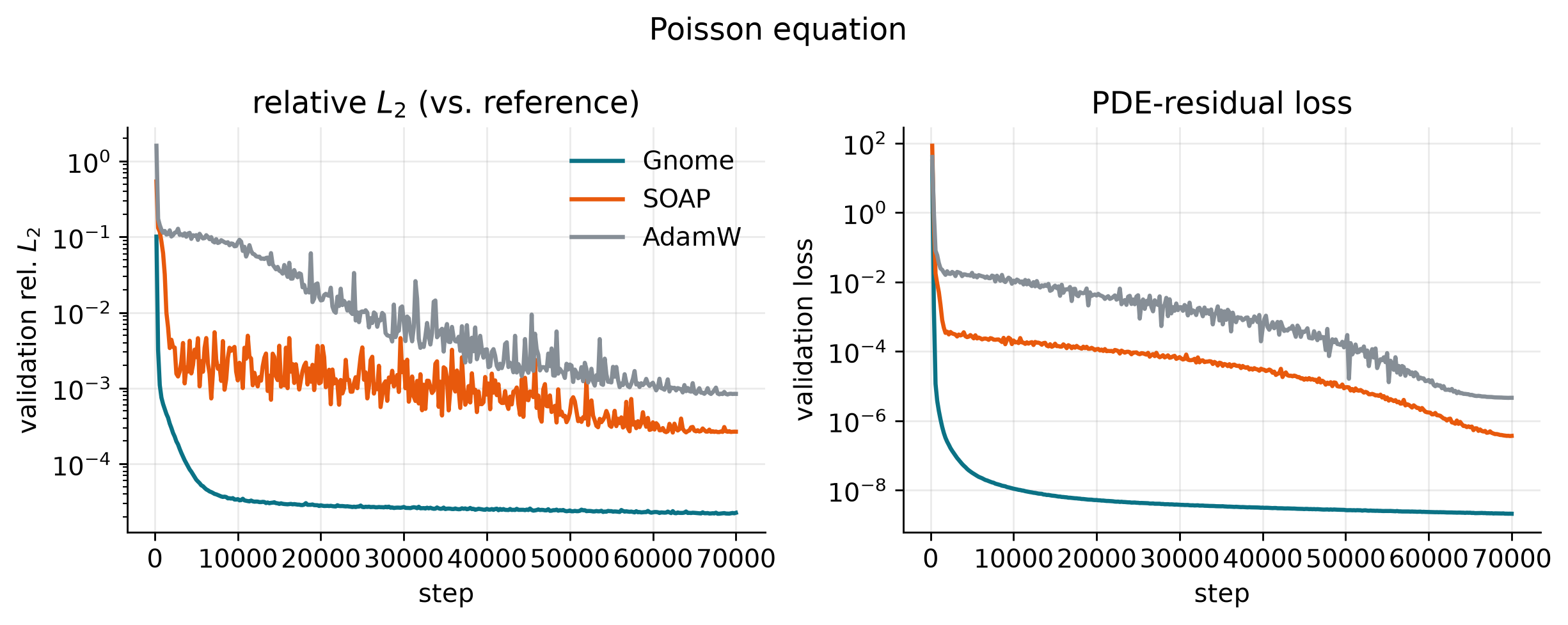
Gnome reaches the lowest error (2.3e-5) at a fixed learning rate; SOAP with a tuned cosine decay is behind at 2.7e-4; AdamW trails at 8.4e-4. The takeaway isn’t the Gnome-vs-SOAP margin here — it’s small and this is the easy problem — it’s that the decay schedule is doing real work for the baselines. Notice also the shape: Gnome descends smoothly and monotonically, while SOAP rattles up and down by an order of magnitude and only settles as its learning rate is annealed away — the same hovering from §1, now driven down by the schedule rather than by the residual. Hold that thought: on Burgers the same schedule is no longer enough.
3.2 Burgers — a shock forms
Viscous Burgers is the canonical first hard PINN: from a smooth initial condition the solution steepens into a near-discontinuity (a shock), and the collocation loss around that shock is exactly the kind of stiff, sharply-curved landscape where a diagonal preconditioner and a global schedule start to struggle. Same setup as before — plain MLP, baselines on warmup + cosine-to-zero, Gnome at fixed LR.
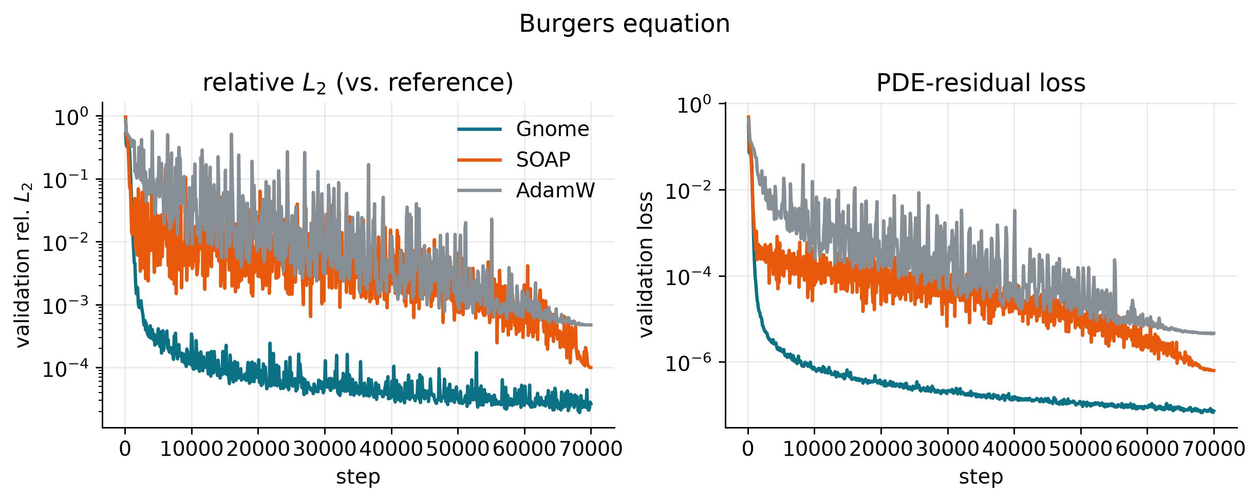
Gnome resolves the shock to a relative \(L_2\) of 2.7e-5 at a fixed learning rate. Both baselines get the full cosine treatment and both land well short: SOAP at 1.0e-4 (roughly 4× Gnome’s error) and AdamW at 4.8e-4 (about 18×). The gap the gentle Poisson problem didn’t show is now open. It’s the same story from §1, one step harder: on Poisson the schedule kept the baselines within a small factor of Gnome; on the stiff Burgers landscape the schedule still helps but no longer closes the gap. And notice the shape again — Gnome’s descent is smooth and monotone while both baselines rattle by an order of magnitude the whole way down, the residual-driven step doing quietly what the schedule does noisily.
Burgers opened the gap on a single stationary shock. Kuramoto–Sivashinsky leans on the same weakness harder — its difficulty is a genuinely stiff operator, not a single localized feature like the shock.
3.3 Kuramoto–Sivashinsky — the stiffest operator
KS is the hardest PDE in this post, and the difficulty is stiffness, not chaos. Its linear part, \(u_{xx} + u_{xxxx}\), spans an enormous range of scales at once: low-wavenumber modes are amplified (the \(k^2\) term, where \(k^2 > k^4\)) while high-wavenumber modes are strongly damped (the \(k^4\) term, \(k^4 \gg k^2\)), and the nonlinear \(u\,u_x\) term couples them together. That fourth-order operator is exactly the kind of wildly anisotropic, ill-conditioned curvature a diagonal preconditioner cannot see — the residual landscape is stiff in the strong sense, and it is where a curvature-aware step earns its keep most clearly.
One deliberate choice: we solve KS only on the early window \(t \in [0, 30]\) and stop short of the chaotic regime. On this large periodic domain (\(L = 32\pi\), the canonical Kassam–Trefethen setup) the solution stays spatially coherent and its energy actually decays through \(t \approx 30\); the coherent structure then destabilizes and breaks up into sustained spatiotemporal chaos near \(t \approx 40\). We do not venture past that breakup, and on purpose. Once the flow is chaotic, sensitive dependence on initial conditions makes a pointwise error against a reference meaningless — two solutions agreeing to eight digits separate to order one within a few dozen time units, so a relative \(L_2\) score would be measuring the chaos, not the optimizer. Staying in the pre-chaotic transient keeps the metric honest while preserving the difficulty we actually care about: the stiffness of the operator.
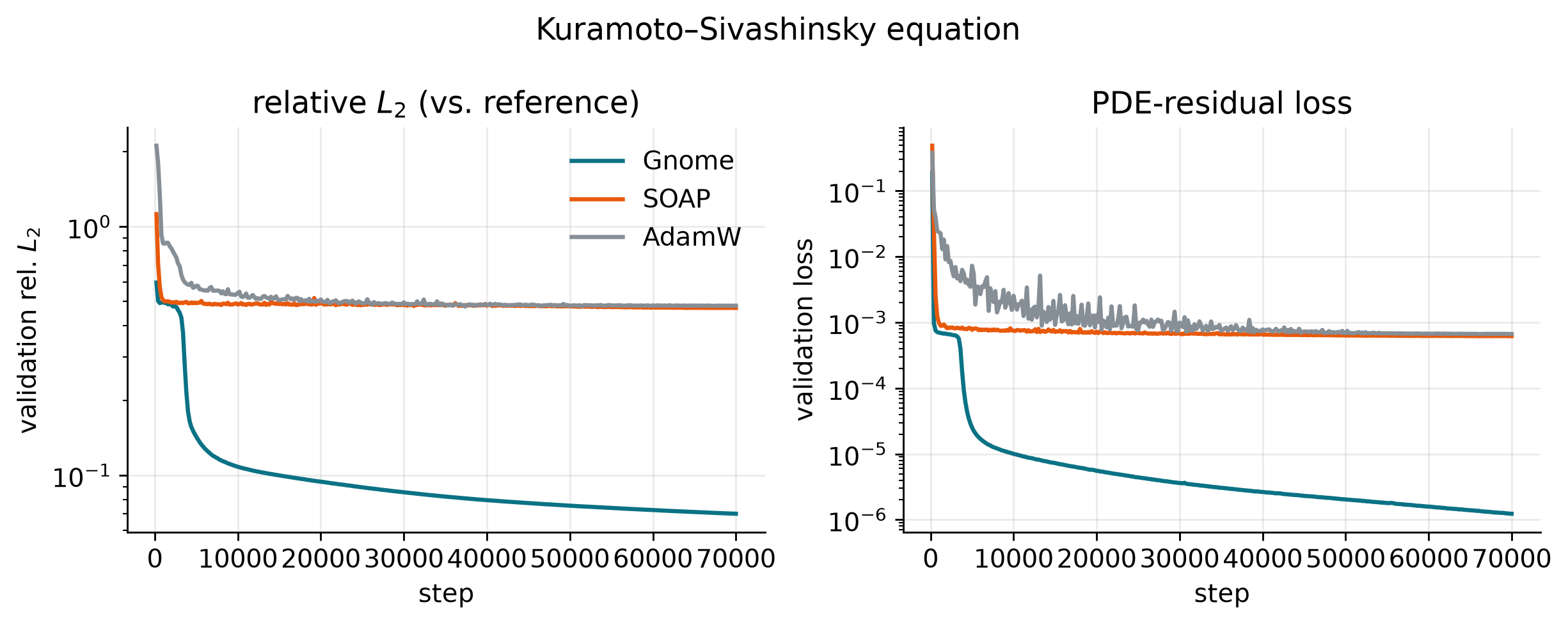
This time the baselines don’t just trail — they never leave the gate. SOAP and AdamW spend all 70,000 steps pinned at a relative \(L_2\) of roughly 0.5 (final: 4.7e-1 and 4.8e-1), and the schedule that kept them competitive on Poisson and merely behind on Burgers buys nothing here. Gnome breaks below 0.3 by step 3,600 and descends to 7.0e-2 — all against the same ETDRK4 reference, on the same tanh MLP and the same collocation points, with only the optimizer changed.
That is the whole arc: the exact denominator pathology from §1 — a step that won’t vanish without a hand-tuned schedule — escalating cleanly across three PDEs. Poisson is gentle enough that the schedule keeps the baselines close; Burgers opens the gap at a shock; and on KS, the stiffest of the three, the baselines fail outright while the residual-driven step converges. Same mechanism, harder problem each time, plainly visible in the metric you actually care about.
4. One real language task: WikiText GPT
Everything in §3 was regression — the \(\sqrt 2\, I\) surrogate. Language modeling is categorical cross-entropy, so this is where §2’s CCE surrogates earn their keep. The WikiText run compares the two: gnome_hutchinson (the analytic square root — every class in every probe) against gnome_fisher (Monte Carlo label sampling — one class per probe). Same optimizer, same basis machinery; the only difference is the variance of the curvature estimate, so the comparison is partly about whether a lower-variance eigenbasis shows up as better training.
The result
We had the compute budget for exactly one real language-modeling task, so here it is: GPT-2 small (124M parameters) on WikiText-103. SOAP and AdamW run on their recommended hyperparameters; the Gnome variants simply borrow SOAP’s, untuned. One logistical note: the Colab sessions hosting these runs disconnected at different points — SOAP earliest, around 19.5k steps — so the plot is capped at 19k, the common window where all four have data.
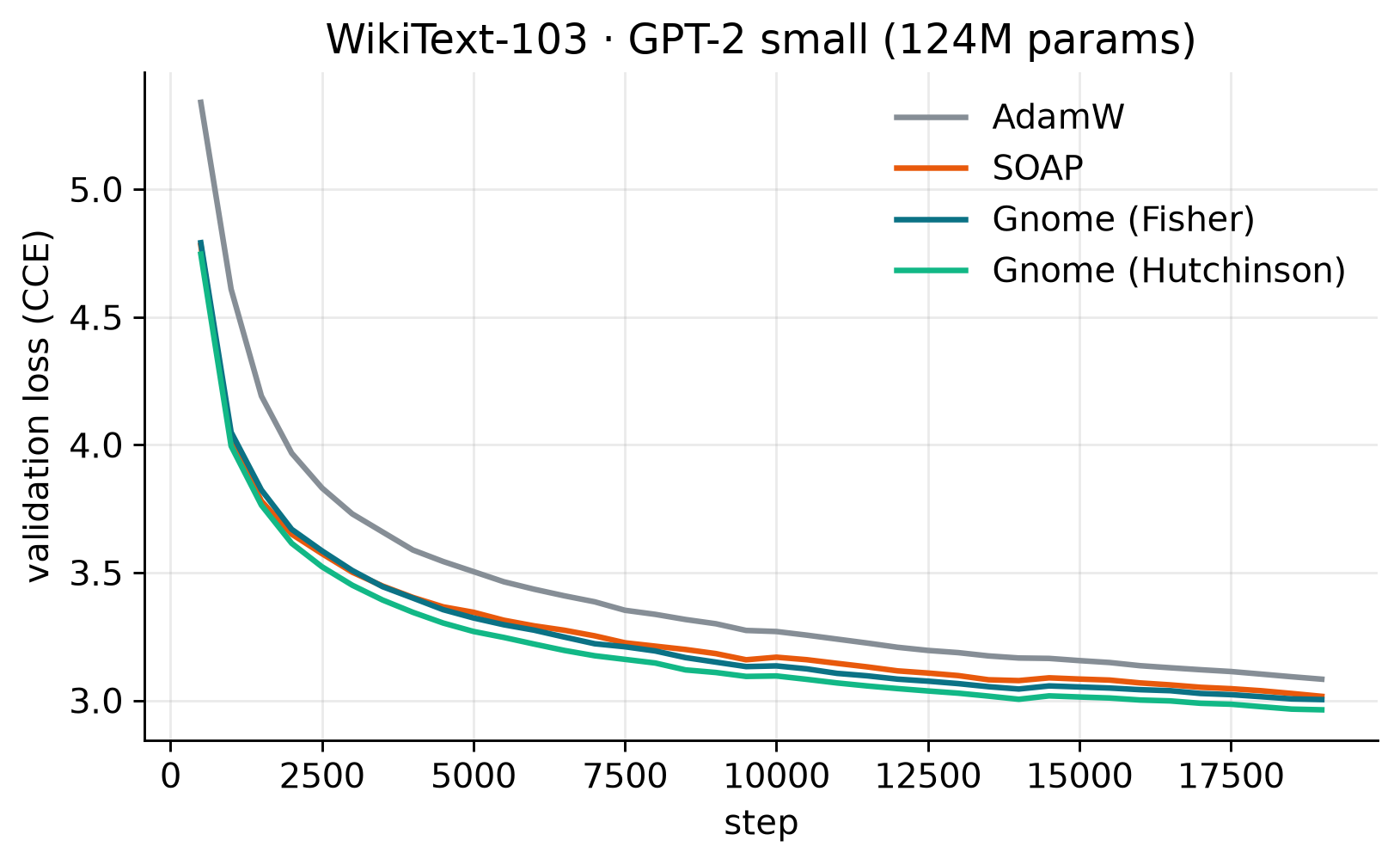
All four train the same 124M-parameter GPT-2. By best validation perplexity the two Gnome variants come out ahead — gnome_hutchinson at 19.4 and gnome_fisher at 20.1, below SOAP (20.4) and AdamW (21.0) — and the Gnome curves also fall faster early. Hutchinson edging Fisher (19.4 vs 20.1) is the small signal §2 predicts: an all-classes-at-once curvature probe has lower variance than a single-sampled-class one, and it shows up as slightly better training.
One model at one scale is not an LLM claim, and we aren’t making one. The point is narrower, and it holds: the GGN story that decides the PINN results doesn’t fall apart the moment you leave regression for cross-entropy — on borrowed, untuned hyperparameters, Gnome lands ahead of both baselines.
One difference from §3: on cross-entropy every optimizer, Gnome included, gets a cosine schedule. The §1 fixed-LR trick is specific to MSE, where the step vanishes because the residual does; cross-entropy gradients don’t vanish at the optimum, so there is no free self-annealing to exploit and Gnome takes the schedule too.
6. Reproducing this
Everything above is regenerated, not transcribed. Each experiment streams an append-only JSONL log to runs/<experiment>/<run_id>.jsonl, and this post is a Quarto document that reads those logs at render time — every figure, every table, and every bolded number in the prose is pulled from the latest completed run on disk. Re-run an experiment and the post updates itself on the next render; delete a run and its numbers degrade to “—” rather than silently going stale.
The code is at github.com/tmayer868/gnome-optimizer, with dependencies managed by uv. One command per experiment:
git clone https://github.com/tmayer868/gnome-optimizer && cd gnome-optimizer
uv sync --extra experiments

uv run python -m experiments.ols_regression              --optimizer gnome --lr 0.1
uv run python -m experiments.poisson_pinn                --optimizer gnome --steps 50000
uv run python -m experiments.burgers_pinn                --optimizer gnome --steps 75000
uv run python -m experiments.kuramoto_sivashinsky_pinn   --optimizer gnome --steps 100000
Swap --optimizer soap or adamw for the baselines. The schedule protocol from §1 is the default: baseline runs get warmup plus cosine decay to zero out of the box, while Gnome ignores the schedule on MSE losses because it self-anneals — so reproducing the comparison requires no flag juggling. (--cosine-decay 1 disables decay for the raw fixed-LR baselines of §1.) The regression and PINN experiments run on CPU, Apple MPS, or CUDA, whichever is available; the WikiText run (§4) needs uv sync --extra llm and a GPU. The README has the full argument lists and the run-artifact format, and docs/method.md has the method details that didn’t fit here.